9 GDP Nowcasting
GDP is published with a lag — typically 6 to 8 weeks after the quarter ends. Nowcasting uses higher-frequency data to estimate GDP in real time, before the official number arrives.
9.1 The nowcasting problem
The fundamental challenge of macroeconomic monitoring is that the variable policymakers care about most — GDP — arrives late and infrequently. The ONS publishes its first estimate of quarterly GDP roughly 40 days after the quarter ends, meaning that for much of any given quarter, the most recent official reading describes an economy that existed three to six months ago. The Bank of England’s Monetary Policy Committee meets eight times per year to set interest rates, and at several of those meetings the latest GDP figure is already stale. The same problem affects fiscal authorities, financial markets, and any analyst who needs to understand the current state of the economy.
The difficulty is compounded by what econometricians call the “ragged edge” problem. Different economic indicators are released on different schedules. Monthly retail sales data might be available through February, industrial production only through January, and labour market figures through December — all at the same calendar date. A nowcasting model must cope with this jagged pattern of data availability, extracting signal from whichever series happen to have been updated most recently. The ragged edge is not a nuisance to be tidied away; it is the defining feature of real-time economic monitoring.
Nowcasting methods range from simple to sophisticated. At one end, bridge equations translate monthly indicators into quarterly GDP estimates using ordinary regression. At the other, dynamic factor models extract latent common factors from dozens of series simultaneously, handling mixed frequencies and missing observations by design. In between sit MIDAS (Mixed Data Sampling) regressions, which use monthly data directly in a quarterly equation by imposing parsimonious weighting schemes on the high-frequency lags. This chapter works through each approach using UK data.
9.2 Bridge equations
The bridge equation is the simplest nowcasting method and remains widely used in central banks and treasuries. The idea is straightforward: take monthly indicators that are correlated with GDP, aggregate them to the quarterly frequency, and use them as regressors in an OLS model for quarterly GDP growth. Because the monthly indicators are released before GDP, the fitted values from this regression constitute a “bridge” from the monthly data to the quarterly target.
The approach works well when a small number of monthly series capture the main drivers of GDP variation. Retail sales proxy household consumption, which accounts for roughly 60 per cent of UK GDP. Industrial production captures the manufacturing and energy sectors. Together, these two indicators often explain a substantial share of quarter-on-quarter GDP movements.
The practical workflow has three steps. First, pull monthly indicators and quarterly GDP from the ONS. Second, aggregate the monthly series to quarterly frequency by taking the within-quarter mean. Third, estimate the bridge equation by OLS and use it to forecast the current quarter.
# Pull quarterly GDP growth (ons_gdp() returns quarter-on-quarter growth by default)
gdp <- ons_gdp() |>
  rename(gdp_growth = value)

# Pull monthly indicators
retail <- ons_retail_sales() |>
  mutate(quarter_date = floor_date(date, "quarter")) |>
  group_by(quarter_date) |>
  summarise(retail_index = mean(value, na.rm = TRUE), .groups = "drop") |>
  mutate(retail_growth = (retail_index / lag(retail_index) - 1) * 100) |>
  rename(date = quarter_date)

# Monthly GDP (proxy for industrial production/services)
monthly_gdp <- ons_monthly_gdp() |>
  mutate(quarter_date = floor_date(date, "quarter")) |>
  group_by(quarter_date) |>
  summarise(monthly_index = mean(value, na.rm = TRUE), .groups = "drop") |>
  mutate(monthly_growth = (monthly_index / lag(monthly_index) - 1) * 100) |>
  rename(date = quarter_date)
With the quarterly-aggregated indicators in hand, merge them with GDP and estimate the bridge equation.
# Merge datasets
bridge_data <- gdp |>
  inner_join(retail, by = "date") |>
  inner_join(monthly_gdp, by = "date") |>
  filter(!is.na(gdp_growth), !is.na(retail_growth), !is.na(monthly_growth))

# Estimate bridge equation
bridge_model <- lm(gdp_growth ~ retail_growth + monthly_growth,
                    data = bridge_data)
summary(bridge_model)
Call:
lm(formula = gdp_growth ~ retail_growth + monthly_growth, data = bridge_data)

Residuals:
      Min        1Q    Median        3Q       Max
-0.235340 -0.070632 -0.005367  0.075464  0.238184

Coefficients:
                 Estimate Std. Error t value Pr(>|t|)
(Intercept)    -0.0003289  0.0092100  -0.036    0.972
retail_growth   0.0022470  0.0062104   0.362    0.718
monthly_growth  0.9965571  0.0061079 163.159   <2e-16 ***
---
Signif. codes:  0 '***' 0.001 '**' 0.01 '*' 0.05 '.' 0.1 ' ' 1

Residual standard error: 0.09699 on 112 degrees of freedom
Multiple R-squared:  0.9986,    Adjusted R-squared:  0.9986
F-statistic: 4.141e+04 on 2 and 112 DF,  p-value: < 2.2e-16
The coefficients tell us how much a one-percentage-point increase in quarterly retail sales growth or monthly GDP growth is associated with higher quarterly GDP growth. The \(R^2\) indicates how much of the quarterly variation these two indicators explain. To produce a nowcast for the current quarter, simply plug in the latest available values of the monthly indicators (aggregated to the quarterly frequency so far) and compute the fitted value.
# Nowcast: use latest available monthly data
# If only 1 or 2 months of the quarter are available, average those
latest_retail_growth <- tail(retail$retail_growth, 1)
latest_monthly_growth <- tail(monthly_gdp$monthly_growth, 1)

nowcast <- predict(bridge_model,
                   newdata = data.frame(retail_growth = latest_retail_growth,
                                        monthly_growth = latest_monthly_growth))
cat("GDP growth nowcast:", round(nowcast, 2), "per cent\n")
GDP growth nowcast: 0.07 per centBridge equations have the virtue of transparency. Every input is observable, every coefficient is interpretable, and the model can be updated in seconds as new monthly data arrive. Their main limitation is that they discard information by aggregating monthly data to the quarterly frequency before estimation. The next two methods address this.
9.3 MIDAS models
Mixed Data Sampling (MIDAS) regressions, developed by Ghysels, Santa-Clara, and Valkanov (2004), avoid the information loss of quarterly aggregation by including the monthly observations directly in the quarterly equation. The key insight is that if a quarter contains three monthly observations, we can include all three as separate regressors — but doing so naively would consume degrees of freedom rapidly. MIDAS solves this by parameterising the weights on the monthly lags with a low-dimensional function, typically the beta or exponential Almon polynomial.
The model takes the form:
\[ y_t^Q = \alpha + \beta \sum_{k=0}^{K} w(k; \theta) x_{t-k/m}^M + \varepsilon_t \]
where \(y_t^Q\) is quarterly GDP growth, \(x^M\) is a monthly indicator, \(m = 3\) is the frequency ratio, and \(w(k; \theta)\) is a weighting function governed by a small number of parameters \(\theta\). The weighting function typically places more weight on recent months and less on distant ones, capturing the intuition that the most recent data are the most informative about the current quarter.
The midasr package in R implements MIDAS regressions with several weighting specifications. The key function is midas_r(), which takes a formula with the mls() (MIDAS lag structure) operator to specify high-frequency regressors.
library(midasr)

# Prepare data in the format midasr expects
# We need monthly and quarterly series that are properly aligned.
# Monthly retail sales growth
retail_monthly <- ons_retail_sales() |>
  arrange(date) |>
  mutate(retail_growth = (value / lag(value) - 1) * 100) |>
  filter(!is.na(retail_growth))

# Align: find date range where both quarterly GDP and monthly retail exist
q_dates <- bridge_data$date
min_date <- max(min(q_dates), floor_date(min(retail_monthly$date), "quarter"))
max_date <- min(max(q_dates), floor_date(max(retail_monthly$date), "quarter"))

y_q <- bridge_data |>
  filter(date >= min_date, date <= max_date) |>
  pull(gdp_growth)

# Extract monthly retail growth for the same quarter range
# midasr needs exactly 3 * length(y_q) monthly obs aligned to the quarters
x_m_df <- retail_monthly |>
  mutate(quarter_date = floor_date(date, "quarter")) |>
  filter(quarter_date >= min_date, quarter_date <= max_date)

# Ensure we have complete quarters only
complete_q <- x_m_df |>
  count(quarter_date) |>
  filter(n == 3) |>
  pull(quarter_date)

y_q <- bridge_data |>
  filter(date %in% complete_q) |>
  pull(gdp_growth)

x_m <- x_m_df |>
  filter(quarter_date %in% complete_q) |>
  arrange(date) |>
pull(retail_growth)The estimated weight function reveals how the model values different monthly lags. If the weights decline steeply, only the most recent month or two matter for the nowcast. If they decline gradually, information from several months back remains useful. Plotting the estimated weights is a standard diagnostic.
# Plot the estimated MIDAS weights
plot_midas_weights <- data.frame(
  lag = 0:8,
  weight = nealmon(coef(midas_model)$x_m, d = 9)
)

ggplot(plot_midas_weights, aes(x = lag, y = weight)) +
  geom_col(fill = "steelblue") +
  labs(title = "MIDAS weight function",
       x = "Monthly lag", y = "Weight") +
  theme_macro()
MIDAS models are particularly useful in the ragged-edge setting. When only one or two months of the current quarter are available, the weighting function automatically adjusts. The model can also be extended to include multiple monthly indicators, each with its own weighting function, giving it the flexibility to handle the mixed-frequency data environment that characterises real-time nowcasting.
9.4 Dynamic factor models
When many monthly indicators are available, a natural question is whether they share a common cyclical component — a single latent “state of the economy” factor that drives co-movement across retail sales, industrial production, employment, and other series. Dynamic factor models (DFMs) formalise this idea. They assume that each observed series is a linear function of a small number of unobserved common factors plus an idiosyncratic component:
\[ X_t = \Lambda F_t + e_t \]
where \(X_t\) is a vector of \(n\) observed indicators, \(F_t\) is a vector of \(r\) common factors (typically \(r = 1\) or \(2\)), \(\Lambda\) is a matrix of factor loadings, and \(e_t\) is idiosyncratic noise. The factors follow a VAR process: \(F_t = \Phi_1 F_{t-1} + \dots + \Phi_p F_{t-p} + \eta_t\). The model is estimated by maximum likelihood via the Kalman filter, which also handles the ragged edge naturally — missing observations at the end of a series are simply integrated out.
The dfms package provides a clean interface for estimating DFMs in R. We begin by assembling a panel of monthly UK indicators. Breadth matters: the more sectors represented, the better the common factor will capture aggregate economic conditions.
library(dfms)

# Pull a panel of monthly UK indicators
retail_sales <- ons_retail_sales() |>
  select(date, retail = value)

monthly_gdp_raw <- ons_monthly_gdp() |>
  select(date, monthly_gdp = value)

unemployment <- ons_unemployment() |>
  select(date, unemployment_rate = value)

employment <- ons_employment() |>
  select(date, employment_rate = value)

wages <- ons_wages() |>
  select(date, wages = value)
# Merge into a panel
panel <- retail_sales |>
full_join(monthly_gdp_raw, by = "date") |>
full_join(unemployment, by = "date") |>
full_join(employment, by = "date") |>
full_join(wages, by = "date") |>
arrange(date) |>
filter(date >= as.Date("2000-01-01"))
# Convert to matrix (dfms expects numeric matrix with dates as rownames)
panel_mat <- panel |>
select(-date) |>
as.matrix()
rownames(panel_mat) <- as.character(panel$date)Before estimating the factor model, each series should be transformed to stationarity (typically by taking log-differences or growth rates) and standardised to have zero mean and unit variance. This ensures that no single series dominates the factor simply because of its scale.
# Transform to growth rates and standardise
panel_growth <- apply(panel_mat, 2, function(x) {
  dx <- c(NA, diff(log(x))) * 100
  (dx - mean(dx, na.rm = TRUE)) / sd(dx, na.rm = TRUE)
})
rownames(panel_growth) <- rownames(panel_mat)

# Estimate dynamic factor model with 1 factor
dfm_model <- DFM(panel_growth, r = 1, p = 2)
summary(dfm_model)
Dynamic Factor Model: n = 5, T = 312, r = 1, p = 2, %NA = 0.3846
Call: DFM(X = panel_growth, r = 1, p = 2)
Summary Statistics of Factors [F]
N Mean Median SD Min Max
f1 312 0.0019 0.051 1.2915 -17.0645 8.0275
Factor Transition Matrix [A]
L1.f1 L2.f1
f1 0.3548 -0.3031
Factor Covariance Matrix [cov(F)]
f1
f1 1.668
Factor Transition Error Covariance Matrix [Q]
u1
u1 1.5188
Observation Matrix [C]
f1
retail 0.5904
monthly_gdp 0.7052
unemployment_rate 0.0675
employment_rate 0.0307
wages 0.1125
Observation Error Covariance Matrix [diag(R) - Restricted]
retail monthly_gdp unemployment_rate employment_rate
0.3669 0.0973 0.9885 0.9951
wages
0.9739
Observation Residual Covariance Matrix [cov(resid(DFM))]
retail monthly_gdp unemployment_rate employment_rate
retail 0.3179 -0.0543* 0.0165 -0.0287
monthly_gdp -0.0543* 0.0222 -0.0183* 0.0110
unemployment_rate 0.0165 -0.0183* 0.9911 -0.5224*
employment_rate -0.0287 0.0110 -0.5224* 0.9981
wages 0.0384 -0.0261* 0.0273 -0.0710
wages
retail 0.0384
monthly_gdp -0.0261*
unemployment_rate 0.0273
employment_rate -0.0710
wages 0.9753
Residual AR(1) Serial Correlation
retail monthly_gdp unemployment_rate employment_rate
-0.16107 -0.01757 0.29153 0.30158
wages
-0.32166
Summary of Residual AR(1) Serial Correlations
N Mean Median SD Min Max
5 0.0186 -0.0176 0.2757 -0.3217 0.3016
Goodness of Fit: R-Squared
retail monthly_gdp unemployment_rate employment_rate
0.6821 0.9778 0.0089 0.0019
wages
0.0247
Summary of Individual R-Squared's
N Mean Median SD Min Max
5 0.3391 0.0247 0.4602 0.0019 0.9778The estimated common factor is an index of broad economic conditions. When it is positive, most indicators are growing above trend; when negative, the economy is contracting. Plotting the factor alongside official GDP growth reveals how well it tracks the business cycle.
# Extract the common factor
# F_pca may have fewer rows if leading NAs were dropped during estimation
n_factor <- nrow(dfm_model$F_pca)
dates_factor <- tail(as.Date(rownames(panel_growth)), n_factor)
factor_ts <- data.frame(
  date = dates_factor,
  factor = dfm_model$F_pca[, 1]
) |>
  filter(!is.na(factor))

# Plot the factor
ggplot(factor_ts, aes(x = date, y = factor)) +
  geom_line(colour = "steelblue") +
  geom_hline(yintercept = 0, linetype = "dashed", colour = "grey50") +
  labs(title = "Estimated common factor from UK monthly indicators",
       x = NULL, y = "Factor value (standardised)") +
  theme_macro()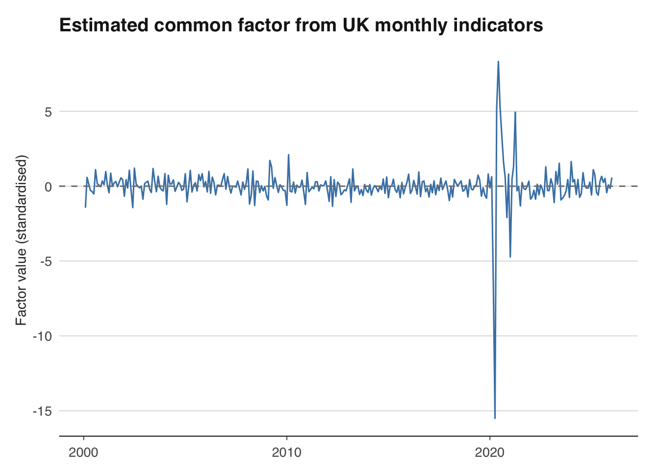
The factor loadings in \(\Lambda\) reveal which indicators are most closely associated with the common cycle. A large positive loading on retail sales, for instance, means that retail sales move strongly with the aggregate factor. The loadings matrix is also useful for diagnosing whether the factor captures a genuine common component or is dominated by a single noisy series.
# Examine factor loadings (stored in C matrix)
loadings_df <- data.frame(
  variable = colnames(panel_growth),
  loading = dfm_model$C[, 1]
)

ggplot(loadings_df, aes(x = reorder(variable, loading), y = loading)) +
  geom_col(fill = "steelblue") +
  coord_flip() +
  labs(title = "Factor loadings", x = NULL, y = "Loading on first factor") +
  theme_macro()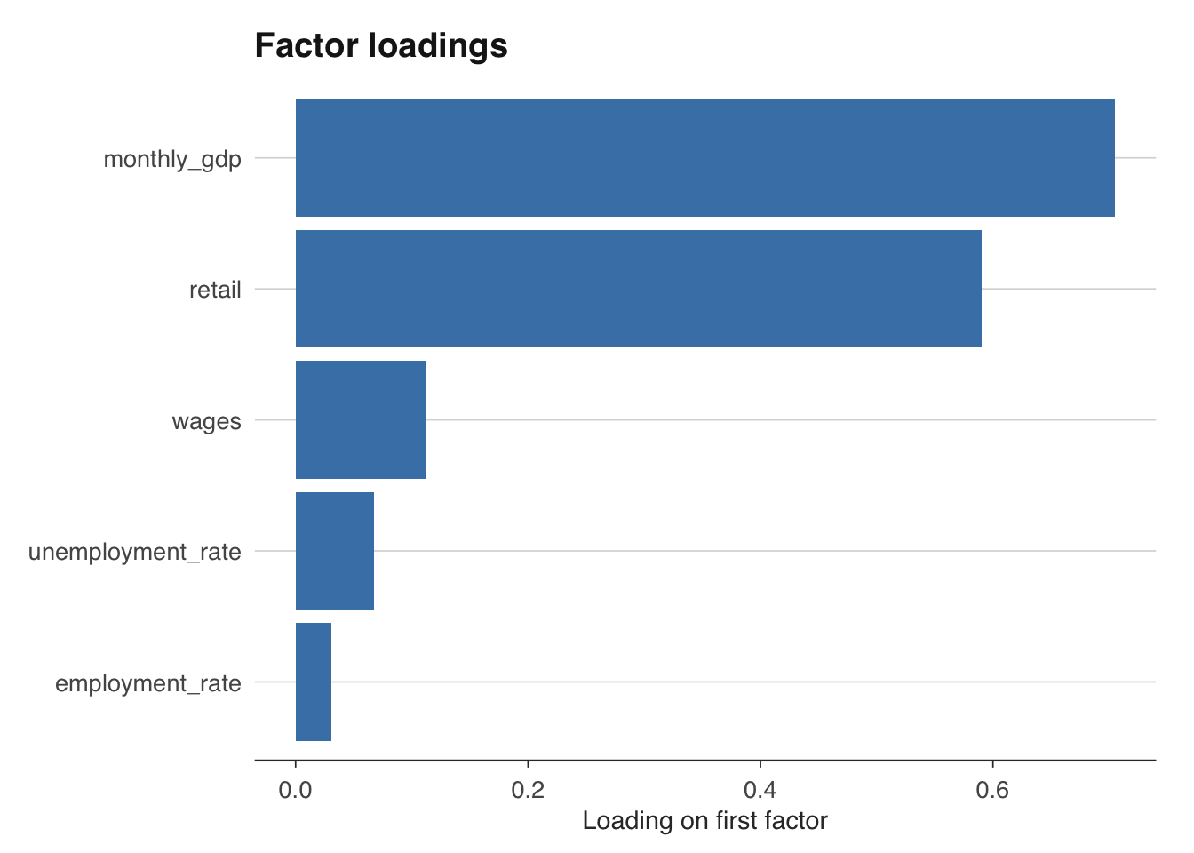
The Kalman smoother within the DFM automatically handles the ragged edge. If retail sales data are available through February but employment data only through January, the model uses whatever information is available to update the factor estimate. This makes DFMs the natural workhorse for institutional nowcasting — the Federal Reserve Bank of New York’s nowcast, for instance, is built on a DFM.
9.5 Building a simple UK GDP nowcaster
The three methods above can be combined into a practical nowcasting workflow. The idea is to maintain a set of models, update them as new data arrive, and produce a combined nowcast that exploits the strengths of each approach. In practice, many institutions use a “model averaging” strategy: take the simple average (or a weighted average based on past performance) of nowcasts from different models.
The workflow has four steps. First, pull all available data and note which series have been updated most recently — this defines the information set. Second, run each model (bridge equation, MIDAS, DFM) on the current data. Third, combine the nowcasts. Fourth, compare to the eventual GDP release once it arrives, and update the model weights accordingly.
# Step 1: Define the information set
cat("Data availability:\n")
cat("Retail sales through:", format(max(retail_monthly$date)), "\n")
cat("Monthly GDP through:", format(max(monthly_gdp$date)), "\n")

# Step 2: Generate nowcasts from each model
nowcast_bridge <- predict(bridge_model,
                          newdata = data.frame(
                            retail_growth = latest_retail_growth,
                            monthly_growth = latest_monthly_growth))

nowcast_midas <- forecast(midas_model, newdata = list(x_m = tail(x_m, 3)))

# DFM nowcast: the last value of the factor, mapped to GDP growth
# via a simple regression of GDP growth on the factor
factor_quarterly <- factor_ts |>
  mutate(quarter_date = floor_date(date, "quarter")) |>
  group_by(quarter_date) |>
  summarise(factor_q = mean(factor, na.rm = TRUE), .groups = "drop") |>
  rename(date = quarter_date)

dfm_bridge <- inner_join(gdp, factor_quarterly, by = "date") |>
  filter(!is.na(gdp_growth))

dfm_reg <- lm(gdp_growth ~ factor_q, data = dfm_bridge)
nowcast_dfm <- predict(dfm_reg,
                       newdata = data.frame(
                         factor_q = tail(factor_quarterly$factor_q, 1)))

# Step 3: Combine
nowcast_combined <- mean(c(nowcast_bridge, nowcast_midas$mean, nowcast_dfm))
cat("\nNowcasts:\n")
cat("Bridge equation:", round(nowcast_bridge, 2), "\n")
cat("MIDAS:", round(nowcast_midas$mean, 2), "\n")
cat("DFM:", round(nowcast_dfm, 2), "\n")
cat("Combined:", round(nowcast_combined, 2), "\n")
An important refinement is pseudo-out-of-sample evaluation. Rather than estimating the model on all available data and reporting the in-sample fit, roll the estimation window forward through time. At each point, estimate the model using only data that would have been available in real time, produce a nowcast, and compare it to the eventual GDP release. This gives an honest assessment of how the nowcaster would have performed historically.
# Pseudo-out-of-sample evaluation for the bridge equation
# Use an expanding window starting from 2015
eval_start <- as.Date("2015-01-01")
eval_data <- bridge_data |> filter(date >= as.Date("2005-01-01"))

results <- data.frame(date = as.Date(character()),
                      actual = numeric(),
                      forecast = numeric())

eval_dates <- eval_data$date[eval_data$date >= eval_start]

for (d in seq_along(eval_dates)) {
  train <- eval_data |> filter(date < eval_dates[d])
  test <- eval_data |> filter(date == eval_dates[d])

  if (nrow(train) < 10 || nrow(test) == 0) next

  m <- lm(gdp_growth ~ retail_growth + monthly_growth, data = train)
  f <- predict(m, newdata = test)

  results <- bind_rows(results,
                       data.frame(date = eval_dates[d],
                                  actual = test$gdp_growth,
                                  forecast = f))
}
9.6 Evaluating forecast accuracy
The standard metrics for evaluating point forecasts are the root mean squared error (RMSE) and mean absolute error (MAE):
\[ \text{RMSE} = \sqrt{\frac{1}{T} \sum_{t=1}^{T} (y_t - \hat{y}_t)^2}, \qquad \text{MAE} = \frac{1}{T} \sum_{t=1}^{T} |y_t - \hat{y}_t| \]
RMSE penalises large errors more heavily than MAE, making it more sensitive to outliers (such as the 2020 Q2 COVID contraction). Both are useful, but for different reasons: RMSE is the natural loss function if you care about variance, while MAE is more robust.
Bridge equation out-of-sample performance:RMSE: 0.114 MAE: 0.09 When comparing two competing models, the Diebold-Mariano test provides a formal statistical framework. The null hypothesis is that the two models have equal predictive accuracy. The test statistic is based on the difference in squared (or absolute) forecast errors.
library(forecast)

# Suppose we have two sets of forecasts
# e1 = errors from model 1, e2 = errors from model 2
e1 <- results$actual - results$forecast  # bridge equation errors

# For comparison, compute a naive forecast (previous quarter's growth)
results_naive <- eval_data |>
  filter(date >= eval_start) |>
  mutate(naive_forecast = lag(gdp_growth))

e2 <- results_naive$gdp_growth - results_naive$naive_forecast
e2 <- e2[!is.na(e2)]

# Diebold-Mariano test
dm_test <- dm.test(e1, e2[seq_along(e1)], alternative = "two.sided")
print(dm_test)
    Diebold-Mariano Test

data:  e1e2[seq_along(e1)]
DM = -1.4552, Forecast horizon = 1, Loss function power = 2, p-value =
0.1529
alternative hypothesis: two.sided
A significant test statistic (small p-value) indicates that one model is genuinely more accurate than the other, not merely luckier over the evaluation sample. In practice, nowcasting models tend to outperform naive benchmarks most clearly during turning points — precisely when the nowcast is most valuable to policymakers.
# Plot actual vs nowcast
ggplot(results, aes(x = date)) +
  geom_line(aes(y = actual, colour = "Actual")) +
  geom_line(aes(y = forecast, colour = "Nowcast"), linetype = "dashed") +
  labs(title = "Bridge equation nowcast vs actual GDP growth",
       x = NULL, y = "Quarter-on-quarter growth (%)",
       colour = NULL) +
  scale_colour_manual(values = c("Actual" = "black", "Nowcast" = "steelblue")) +
  theme_macro()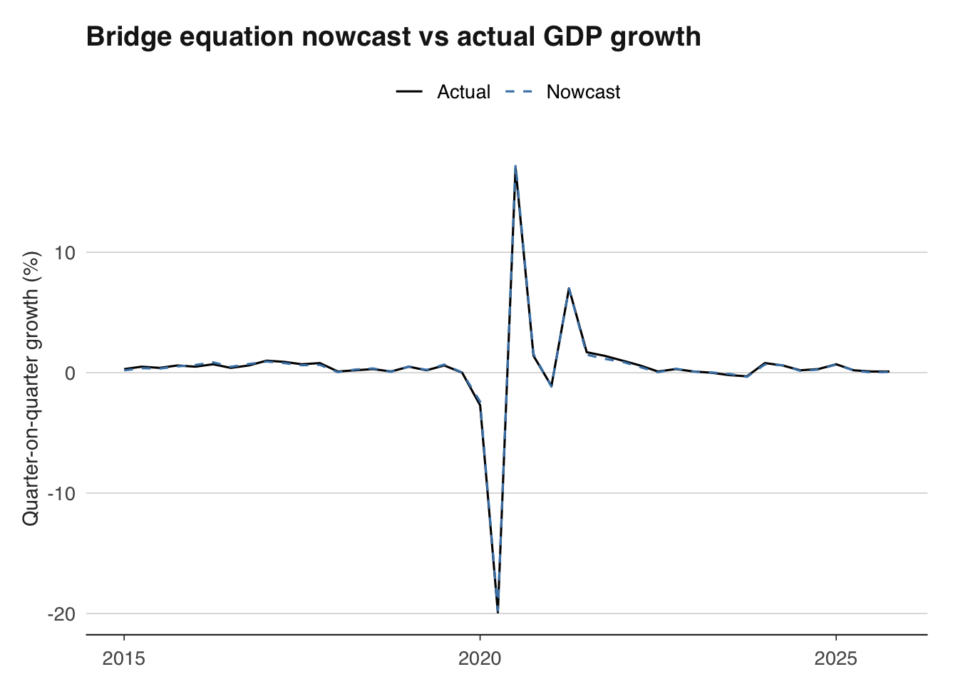
The chart above reveals where the nowcaster succeeds and fails. Systematic over- or under-prediction suggests model misspecification. Large errors clustered around specific episodes (recessions, pandemics) suggest that the model struggles with structural breaks — a common limitation of linear nowcasting methods that motivates the more flexible approaches covered in advanced treatments.
9.7 Exercises
Build a bridge equation that uses monthly retail sales and industrial production to predict quarterly GDP growth. How accurate is it out of sample?
Estimate a dynamic factor model using
dfmswith 5 monthly UK indicators. What share of variation does the first factor explain?Compare your nowcast for the latest quarter against the Bank of England’s published nowcast (from the Monetary Policy Report). How close are they?