---
execute:
eval: true
---
# Cross-Country Comparisons {#sec-cross-country}
Why are some countries richer than others? This is arguably the most important question in economics. A child born in Norway can expect an income roughly 50 times higher than one born in the Democratic Republic of Congo. Understanding what drives these differences — and whether they are converging or diverging — is the domain of growth economics.
This chapter covers three pillars of cross-country analysis: the convergence hypothesis (do poor countries catch up?), growth accounting (what are the proximate sources of growth?), and institutions (what are the fundamental causes?). We then introduce panel data techniques that allow us to estimate these relationships rigorously using data from many countries over many years.
## The convergence hypothesis
The Solow growth model makes a powerful prediction: poorer countries should grow faster than richer ones. The logic is diminishing returns to capital. A country with very little capital per worker gets a large output boost from each additional unit of investment, while a capital-rich country gets a smaller boost. If all countries have access to the same technology and save at similar rates, they should converge to the same steady-state income level. This is **unconditional convergence** — the prediction that initial income alone predicts subsequent growth, regardless of other characteristics.
**Conditional convergence** is a weaker but more defensible prediction. It says that countries converge to their own steady states, which depend on savings rates, population growth, human capital, and institutional quality. Two countries with identical fundamentals but different starting points will converge. But two countries with different fundamentals may diverge, even if one starts poorer. The empirical implication is that initial income should predict growth only after controlling for these other factors.
Let us test unconditional convergence using World Bank data. We need GDP per capita in constant dollars for a large panel of countries, with observations in 1990 and 2020.
```{r}
library(WDI)
library(dplyr)
library(tidyr)
library(ggplot2)
source("../R/theme_macro.R")

# Download GDP per capita (constant 2015 US$)
gdp_pc <- WDI(
  indicator = c(gdp_pc = "NY.GDP.PCAP.KD"),
  start = 1990, end = 2020,
  extra = TRUE
)

# Keep only countries (not aggregates like "World" or "OECD")
gdp_pc <- gdp_pc |>
  filter(region != "Aggregates")

# Get initial (1990) GDP per capita and average annual growth
convergence <- gdp_pc |>
  filter(year %in% c(1990, 2020)) |>
  select(iso3c, country, year, gdp_pc) |>
  pivot_wider(names_from = year, values_from = gdp_pc, names_prefix = "y") |>
  filter(!is.na(y1990), !is.na(y2020), y1990 > 0) |>
  mutate(
    avg_growth = ((y2020 / y1990)^(1/30) - 1) * 100,
    log_initial = log(y1990)
  )

nrow(convergence)
```
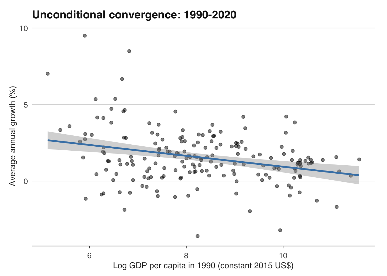
Now plot the classic convergence chart: log initial GDP per capita on the x-axis, average annual growth on the y-axis. If unconditional convergence holds, we should see a downward-sloping relationship — poorer countries (lower initial GDP) growing faster (higher average growth).
```{r}
ggplot(convergence, aes(x = log_initial, y = avg_growth)) +
  geom_point(alpha = 0.5) +
  geom_smooth(method = "lm", se = TRUE, colour = "steelblue") +
  labs(
    title = "Unconditional convergence: 1990-2020",
    x = "Log GDP per capita in 1990 (constant 2015 US$)",
    y = "Average annual growth (%)"
  ) +
  theme_macro()
```
```{r}
# Fit the regression
convergence_model <- lm(avg_growth ~ log_initial, data = convergence)
summary(convergence_model)
```
The result is typically weak. The coefficient on log initial GDP per capita is often statistically insignificant or only marginally significant, and the $R^2$ is very low — usually below 0.05. Unconditional convergence does not hold in the full sample. Some poor countries have grown rapidly (China, India, Vietnam), but many others have stagnated or even regressed (much of sub-Saharan Africa, several post-Soviet states).
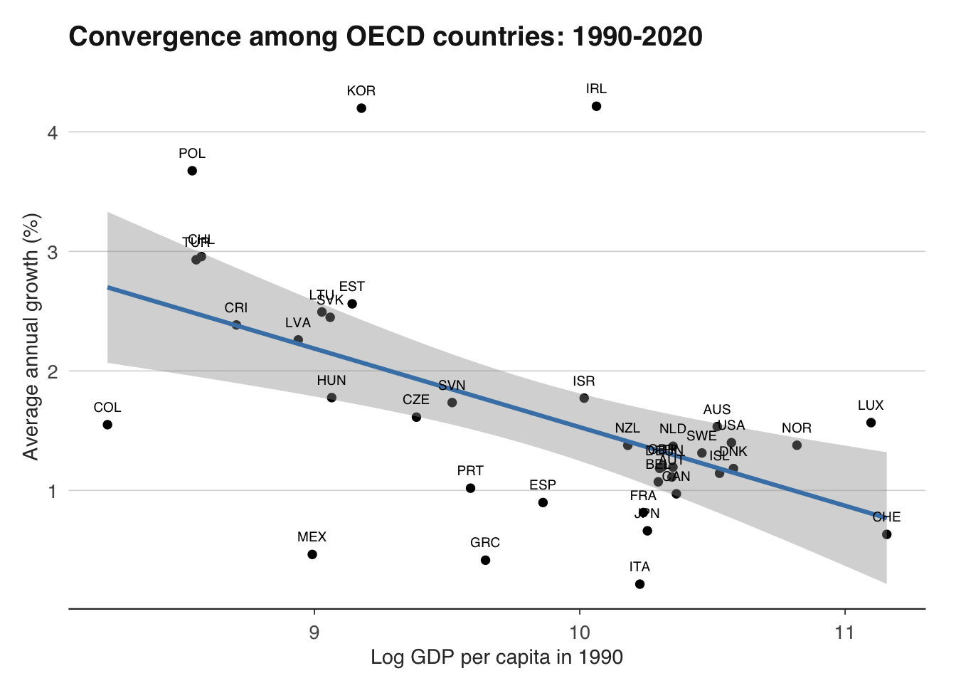
However, if we restrict the sample to OECD countries — a more homogeneous group with broadly similar institutions and policies — convergence is much stronger. Ireland, South Korea, and Poland have grown rapidly from relatively low starting points, while the United States and Switzerland have grown more slowly from high ones.
```{r}
# Convergence among OECD countries only
oecd <- c("AUS", "AUT", "BEL", "CAN", "CHL", "COL", "CRI", "CZE",
          "DNK", "EST", "FIN", "FRA", "DEU", "GRC", "HUN", "ISL",
          "IRL", "ISR", "ITA", "JPN", "KOR", "LVA", "LTU", "LUX",
          "MEX", "NLD", "NZL", "NOR", "POL", "PRT", "SVK", "SVN",
          "ESP", "SWE", "CHE", "TUR", "GBR", "USA")

convergence_oecd <- convergence |>
  filter(iso3c %in% oecd)

ggplot(convergence_oecd, aes(x = log_initial, y = avg_growth)) +
  geom_point() +
  geom_smooth(method = "lm", se = TRUE, colour = "steelblue") +
  geom_text(aes(label = iso3c), size = 2.5, nudge_y = 0.15) +
  labs(
    title = "Convergence among OECD countries: 1990-2020",
    x = "Log GDP per capita in 1990",
    y = "Average annual growth (%)"
  ) +
  theme_macro()
```
This is the core insight of Mankiw, Romer, and Weil (1992): convergence is conditional. Countries converge, but only towards their own steady states. To explain cross-country income differences, we need to understand what determines those steady states — which brings us to growth accounting and institutions.
## Growth accounting
Growth accounting decomposes the growth rate of output into contributions from capital, labour, and a residual called Total Factor Productivity (TFP). The framework starts with a Cobb-Douglas production function:
$$Y = A \cdot K^{\alpha} \cdot L^{1-\alpha}$$
where $Y$ is output, $A$ is TFP, $K$ is the capital stock, $L$ is the labour input, and $\alpha$ is capital's share of income (typically around 0.3 for developed economies). Taking logarithms and differentiating with respect to time gives us the growth accounting equation:
$$g_Y = g_A + \alpha \cdot g_K + (1-\alpha) \cdot g_L$$
That is: output growth ($g_Y$) equals TFP growth ($g_A$) plus the weighted contributions of capital growth ($g_K$) and labour growth ($g_L$). TFP is calculated as the residual — the portion of output growth not explained by the growth of measured inputs:
$$g_A = g_Y - \alpha \cdot g_K - (1-\alpha) \cdot g_L$$
TFP is sometimes called the "measure of our ignorance." It captures everything that raises output beyond what can be attributed to more capital and more labour: technological progress, better management, improved institutions, more efficient resource allocation, and measurement error. Despite being a residual, TFP is typically the largest contributor to long-run growth in developed economies — accounting for 50–70 per cent of growth in the US and UK since 1950.
We can perform a simple growth accounting exercise for the UK using ONS productivity data:
```{r}
library(ons)

# ONS publishes output per hour and per worker indices
productivity <- ons_productivity()

head(productivity)
```
```{r}
# Alternatively, construct a manual growth accounting exercise
# using GDP, capital stock, and employment data

# GDP growth (ons_gdp() returns quarterly growth rates by default)
gdp <- ons_gdp() |>
  arrange(date)

# Employment
employment <- ons_employment()

# For capital stock, use the ONS capital stocks dataset
# or approximate using gross fixed capital formation

# Simple annual growth accounting:
# Suppose we have annual: gdp_growth, capital_growth, labour_growth
# alpha <- 0.3
# tfp_growth <- gdp_growth - alpha * capital_growth - (1 - alpha) * labour_growth
```
For a more detailed decomposition, the ONS publishes an official multi-factor productivity release that breaks output growth into contributions from labour composition (quality), capital deepening (quantity and quality of capital per worker), and multi-factor productivity. This is available in the "Multi-factor productivity" statistical bulletin.
```{r}
# Stylised UK growth accounting (average annual, per cent)
library(tibble)

uk_growth <- tibble(
  period = c("1990-2000", "2000-2007", "2007-2019", "2019-2023"),
  gdp_growth = c(2.8, 2.5, 1.5, 0.8),
  capital_contribution = c(0.9, 0.8, 0.5, 0.3),
  labour_contribution = c(0.5, 0.6, 0.7, 0.3),
  tfp_growth = c(1.4, 1.1, 0.3, 0.2)
)

uk_growth |>
  pivot_longer(-period, names_to = "component", values_to = "pct") |>
  filter(component != "gdp_growth") |>
  ggplot(aes(x = period, y = pct, fill = component)) +
  geom_col(position = "stack") +
  scale_fill_macro() +
  labs(
    title = "UK growth accounting by decade",
    x = NULL, y = "Contribution to GDP growth (pp)",
    fill = NULL
  ) +
  theme_macro()
```
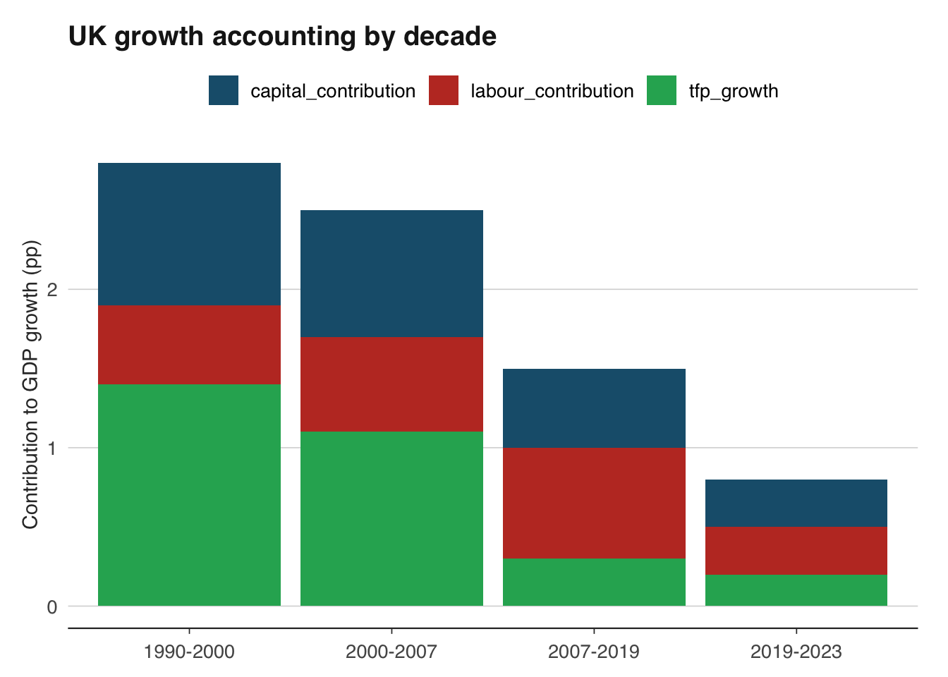
The pattern reveals the UK's "productivity puzzle." Before the financial crisis, TFP growth was the dominant source of output growth — averaging over 1 per cent per year. After 2007, TFP growth collapsed to near zero. Labour input remained positive (employment rose strongly after 2012), and capital deepening continued, but without TFP growth, overall GDP growth was anaemic. This productivity slowdown is the single most important macroeconomic development in the UK since the financial crisis, and explaining it remains an open question. Leading candidates include weak business investment, reduced labour mobility, the long tail of banking sector damage, slower technology diffusion, and measurement issues in the digital economy.
The productivity puzzle is not unique to the UK. The United States, the euro area, and Japan all experienced a marked slowdown in TFP growth after 2005–2008. Robert Gordon's "The Rise and Fall of American Growth" (2016) argues that the period of rapid TFP growth (1920–1970) was historically anomalous, driven by one-off inventions (electricity, the internal combustion engine, indoor plumbing) that cannot be repeated. Others, like Erik Brynjolfsson, argue that we are in a period of "measured" slowdown but unmeasured acceleration, as digital technologies transform production in ways that GDP statistics fail to capture.
## Institutions and growth
Why does growth accounting leave so much unexplained? Because capital, labour, and even TFP are proximate causes of growth — they describe *how* a country grows but not *why*. A deeper question is: why do some countries accumulate more capital, invest more in human capital, and deploy technology more efficiently than others?
Daron Acemoglu, Simon Johnson, and James Robinson — in a series of influential papers and their book "Why Nations Fail" (2012) — argue that the fundamental cause is **institutions**: the rules, norms, and enforcement mechanisms that shape economic incentives. Countries with "inclusive" institutions — secure property rights, impartial courts, competitive markets, constraints on executive power — create incentives for investment, innovation, and effort. Countries with "extractive" institutions — where elites can confiscate wealth, rig markets, or suppress competition — discourage productive activity and encourage rent-seeking.
The empirical challenge is that institutions and income are endogenous: rich countries can afford better institutions, and better institutions may cause higher income. Acemoglu, Johnson, and Robinson address this with an instrumental variables strategy using settler mortality rates in former colonies — but the debate over identification continues.
We can examine the correlation between institutional quality and GDP per capita using the World Bank's Worldwide Governance Indicators (WGI), which measure six dimensions of governance: voice and accountability, political stability, government effectiveness, regulatory quality, rule of law, and control of corruption.
```{r}
# Download GDP per capita
gdp_data <- WDI(
  indicator = c(gdp_pc = "NY.GDP.PCAP.KD"),
  start = 2020, end = 2020,
  extra = TRUE
) |>
  filter(region != "Aggregates", !is.na(gdp_pc))

# World Governance Indicators can be downloaded from:
# https://info.worldbank.org/governance/wgi/
# The WDI package also provides some governance indicators

wgi <- WDI(
  indicator = c(
    rule_of_law = "RL.EST",
    govt_effectiveness = "GE.EST",
    control_corruption = "CC.EST"
  ),
  start = 2020, end = 2020
)

# Merge
institutions <- gdp_data |>
  inner_join(wgi, by = c("iso2c", "year")) |>
  filter(!is.na(rule_of_law), !is.na(gdp_pc))

nrow(institutions)
```
```{r}
ggplot(institutions, aes(x = rule_of_law, y = log(gdp_pc))) +
  geom_point(alpha = 0.5) +
  geom_smooth(method = "lm", se = TRUE, colour = "steelblue") +
  labs(
    title = "Rule of law and GDP per capita (2020)",
    x = "Rule of Law index (WGI)",
    y = "Log GDP per capita (constant 2015 US$)"
  ) +
  theme_macro()
```
```{r}
# Cross-section regression
inst_model <- lm(log(gdp_pc) ~ rule_of_law + control_corruption,
                 data = institutions)
summary(inst_model)
```
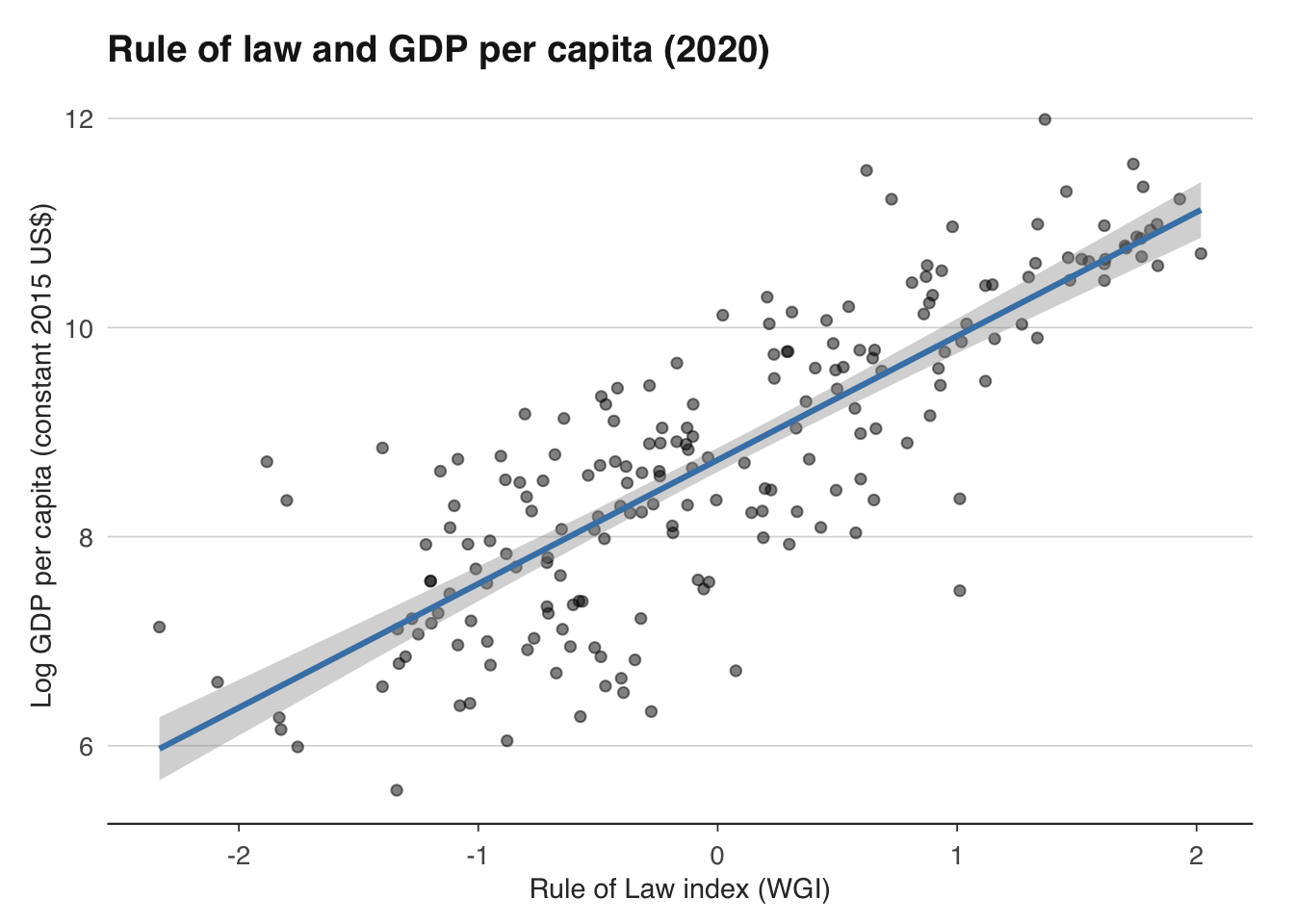
The correlation is strikingly strong — typically $R^2 > 0.5$ in a simple bivariate regression of log GDP per capita on rule of law. But correlation is not causation. Several objections arise immediately. First, reverse causality: richer countries have more resources to build courts, train judges, and fight corruption. Second, omitted variables: geography, culture, colonial history, and natural resources all correlate with both institutions and income. Third, measurement error: governance indicators are partly based on perceptions of business executives and experts, who may rate countries higher simply because they are richer.
Despite these caveats, the institutional explanation has become the dominant paradigm in growth economics. The Nobel Prize in Economics was awarded to Acemoglu, Johnson, and Robinson in 2024 for their work on how institutions shape prosperity. The policy implication is profound but daunting: if institutions are the binding constraint on development, then aid and investment alone are insufficient — what matters is governance reform, which is politically difficult and historically slow.
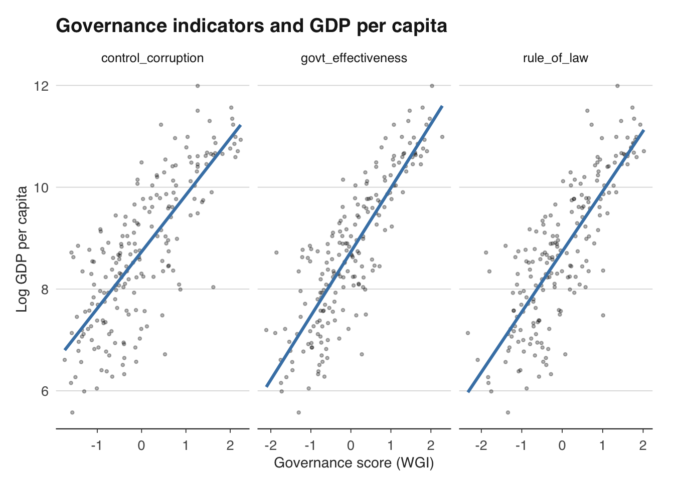
```{r}
# Visualise all three governance dimensions
institutions |>
  select(country.x, gdp_pc, rule_of_law, govt_effectiveness, control_corruption) |>
  pivot_longer(
    cols = c(rule_of_law, govt_effectiveness, control_corruption),
    names_to = "indicator",
    values_to = "score"
  ) |>
  ggplot(aes(x = score, y = log(gdp_pc))) +
  geom_point(alpha = 0.3, size = 0.8) +
  geom_smooth(method = "lm", se = FALSE, colour = "steelblue") +
  facet_wrap(~indicator, scales = "free_x") +
  labs(
    title = "Governance indicators and GDP per capita",
    x = "Governance score (WGI)", y = "Log GDP per capita"
  ) +
  theme_macro()
```
## Panel data techniques for macro
Cross-sectional regressions — one observation per country — suffer from omitted variable bias. Every country differs in countless ways (geography, history, culture, resources), and no set of controls can capture all of them. Panel data, which observe the same countries over multiple time periods, offer a powerful solution: **fixed effects**.
A country fixed effect absorbs all time-invariant characteristics of that country — its geography, colonial history, deep cultural traits, and anything else that does not change over the sample period. This means that fixed effects estimates are identified purely from *within-country variation over time*. If a country's institutional quality improves over a decade, does its growth also improve? This is a much cleaner comparison than asking whether countries with better institutions are richer, because it removes all the static confounders.
The fixed effects model for a panel of countries $i$ over time periods $t$ is:
$$y_{it} = \alpha_i + \beta \cdot x_{it} + \gamma_t + \varepsilon_{it}$$
where $\alpha_i$ is the country fixed effect, $\gamma_t$ is a time fixed effect (absorbing global shocks like the 2008 financial crisis that affect all countries), $x_{it}$ is a vector of time-varying explanatory variables, and $\varepsilon_{it}$ is the error term. The coefficients $\beta$ are identified from within-country, within-time-period variation.
In R, the `fixest` package provides a fast and elegant implementation of fixed effects estimation via `feols()`. The `plm` package is an older alternative. We will use `fixest`.
```{r}
library(WDI)
library(dplyr)

# Download panel data for OECD countries
panel_raw <- WDI(
  indicator = c(
    growth = "NY.GDP.MKTP.KD.ZG",        # GDP growth
    investment = "NE.GDI.TOTL.ZS",        # Gross capital formation (% GDP)
    trade = "NE.TRD.GNFS.ZS",            # Trade (% GDP)
    govt_effectiveness = "GE.EST",         # Government effectiveness
    population_growth = "SP.POP.GROW"      # Population growth
  ),
  start = 2000, end = 2020,
  extra = TRUE
)

# Filter to OECD countries
oecd_codes <- c("AUS", "AUT", "BEL", "CAN", "CHL", "COL", "CZE", "DNK",
                "EST", "FIN", "FRA", "DEU", "GRC", "HUN", "ISL", "IRL",
                "ISR", "ITA", "JPN", "KOR", "LVA", "LTU", "LUX", "MEX",
                "NLD", "NZL", "NOR", "POL", "PRT", "SVK", "SVN", "ESP",
                "SWE", "CHE", "TUR", "GBR", "USA")

panel <- panel_raw |>
  filter(iso3c %in% oecd_codes) |>
  select(iso3c, year, growth, investment, trade,
         govt_effectiveness, population_growth)

# Check coverage
panel |>
  summarise(
    countries = n_distinct(iso3c),
    years = n_distinct(year),
    obs = n(),
    complete = sum(complete.cases(pick(everything())))
  )
```
Now estimate the panel regression with country and year fixed effects:
```{r}
library(fixest)

# Two-way fixed effects: country + year
fe_model <- feols(
  growth ~ investment + trade + govt_effectiveness + population_growth |
    iso3c + year,
  data = panel
)

summary(fe_model)
```
Interpreting the coefficients: the estimate on `investment` tells us that, *within a given OECD country*, a one-percentage-point increase in the investment rate is associated with a certain change in GDP growth, holding constant trade openness, governance, and population growth — and after removing country-specific and year-specific effects. This is a much more credible estimate than a cross-sectional regression, because it is not confounded by the myriad time-invariant differences between, say, Luxembourg and Mexico.
The year fixed effects ($\gamma_t$) are important for macro panels. Without them, a global recession like 2008–2009 would create a spurious negative correlation between growth and any variable that happened to be low in those years. Year fixed effects absorb all common shocks, ensuring that the estimates reflect only country-specific variation.
An alternative to fixed effects is **random effects**, which assumes that country-specific effects are uncorrelated with the explanatory variables. This is a stronger assumption but allows estimation of the effects of time-invariant variables (like geography or colonial history). The **Hausman test** compares fixed and random effects estimates: if they differ significantly, the random effects assumption is violated and fixed effects should be preferred.
```{r}
# Random effects model for comparison
library(plm)

# Convert to a plm panel data frame
panel_plm <- pdata.frame(
  panel |> filter(complete.cases(pick(growth, investment, trade,
                                       population_growth))),
  index = c("iso3c", "year")
)

# Random effects
re_model <- plm(
  growth ~ investment + trade + population_growth,
  data = panel_plm,
  model = "random"
)

# Fixed effects (within estimator)
fe_model_plm <- plm(
  growth ~ investment + trade + population_growth,
  data = panel_plm,
  model = "within"
)

# Hausman test: H0 is that RE is consistent (i.e., RE is fine)
phtest(fe_model_plm, re_model)
```
If the Hausman test rejects (p-value < 0.05), the random effects estimates are inconsistent and we should use fixed effects. In macro panels, this is almost always the case — country-specific effects (institutions, geography, culture) are almost certainly correlated with the explanatory variables. Fixed effects is the workhorse estimator for macro panel data.
A few practical cautions for panel regressions in macroeconomics. First, standard errors should be clustered at the country level to account for serial correlation within countries — `fixest` does this by default when you include fixed effects. Second, macro panels are "short and wide" (20–30 years, 30–40 countries), which limits the precision of estimates. Third, many macro variables are persistent (GDP growth, investment rates), raising concerns about Nickell bias in dynamic panels. For dynamic specifications, the Arellano-Bond GMM estimator is standard, but its small-sample properties are poor when the number of time periods is close to the number of countries.
```{r}
# Clustered standard errors (fixest does this by default with FEs)
# But we can be explicit:
fe_robust <- feols(
  growth ~ investment + trade + population_growth | iso3c + year,
  data = panel,
  cluster = ~iso3c
)

# Compare standard errors
etable(fe_model, fe_robust, se = "cluster")
```
## Exercises
1. Using the `WDI` package, download GDP per capita for all countries in 1990 and 2020. Test the unconditional convergence hypothesis by regressing average annual growth on log initial GDP per capita. Is the slope statistically significant? What is the $R^2$? Repeat for OECD countries only. How do the results differ?
2. Perform a growth accounting exercise for the UK using ONS data. Assume $\alpha = 0.3$. If UK GDP grew at 1.5 per cent per year over 2010–2019, capital grew at 1.8 per cent, and labour grew at 0.8 per cent, what was TFP growth? What share of total growth does each factor account for?
3. Download the World Bank's Worldwide Governance Indicators for 2020. Plot log GDP per capita against each of the six governance dimensions. Which dimension has the strongest correlation with income? Run a multiple regression with all six dimensions — how does multicollinearity affect the results?
4. Estimate a panel regression of GDP growth on investment, trade openness, and population growth for OECD countries over 2000–2020, using both fixed effects and random effects. Conduct a Hausman test. Which model is preferred? Interpret the coefficient on investment.
5. The convergence regression $g_i = \alpha + \beta \cdot \ln(y_{i,0}) + \varepsilon_i$ implies a convergence speed of $-\beta$ per year. If $\beta = -0.02$, how many years does it take for a country to close half the gap to its steady state? (Hint: the half-life is $\ln(2) / |\beta|$.) Is this fast or slow in practice?